An array offers fast access, but inserting or deleting an element often means shifting a large number of items around — the cost isn’t as small as it looks. A linked list flips that trade-off: it gives up contiguous memory in exchange for flexible insertion and deletion. Elements are no longer located by index, but by a pointer each node stores itself, chaining one to the next. This post starts from the basic structure of a linked list, working through the trade-off against arrays and the real complexity behind each operation.
Definition: Linked List
A linked list is a data structure in which objects are arranged in linear order. Unlike an array, where that order is determined by index values, a linked list’s order is determined by a pointer stored inside each object. The list is made up of a chain of nodes, and each node has two fields:
- Data field: stores the actual data the node holds
- Link field: a pointer to the next node
Because the elements of a linked list usually carry a searchable key, a linked list is sometimes also called a search list. As a data structure, it’s also commonly used to implement a dynamic set — a set that supports frequent insertion and deletion. This is the core trade-off between a linked list and an array: an array gives up flexible insertion and deletion in exchange for random access, while a linked list does the opposite.
Singly Linked List
As mentioned above, what makes a linked list distinctive is that it chains individual nodes together, with each node holding both data and a pointer.
This section covers the singly linked list; the doubly linked list comes later — each serves its own purpose.
Initializing a Linked List
Before initializing a linked list, we first need to define a node:
1 | class ListNode: |
A list is like an unfolded string of beads — it always has a front and a back. The front is called the head, and the back is called the tail. So we can try building a list like this:
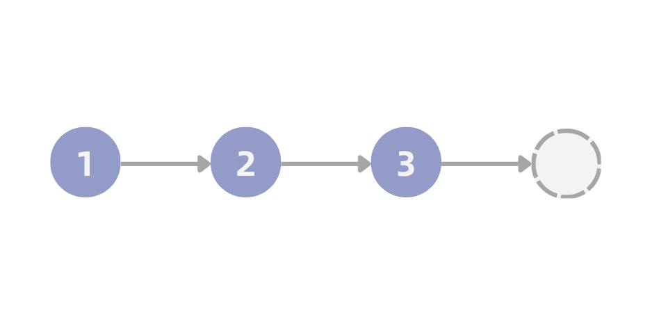
Implemented in Python, that looks like:
1 | head = ListNode(1) |
Notice that since 3 is the very end of the list, its next node is None.
Traversing Nodes
Traversal means starting from the head node and moving forward one node at a time via the next attribute, until you hit None — which means you’ve reached the end of the list and there’s no next node.
When traversing, we typically use curr to keep track of where we currently are, and use a loop to move it forward:
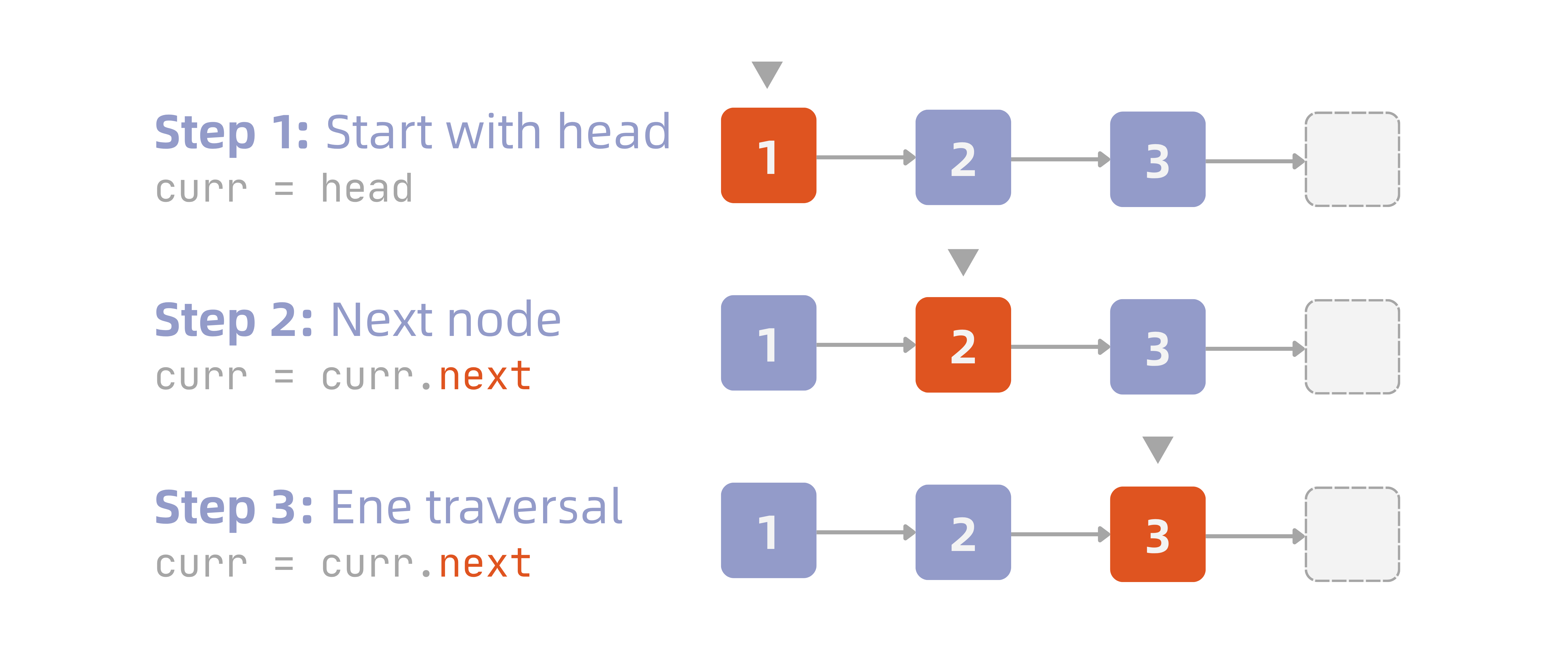
The implementation looks like this:
1 | def traverse(head: ListNode | None) -> None: |
One thing to watch out for: the loop condition must not be written as curr.next is not None — that would stop right at the tail node (since its next is None). Printing one value per line isn’t very readable either, though, so let’s rewrite the traverse function a bit:
1 | def traverse(head: ListNode | None) -> str: |
Printed, this gives:
1 | '1 -> 2 -> 3' |
Separately, if you want to work out the length of a list, you can use a count variable while traversing:
1 | def length(head: ListNode | None) -> int: |
Inserting a ListNode
Inserting a node breaks down into three cases: inserting at the head, inserting after a given node, and inserting at the tail.
Inserting at the Head
The new node needs to become the new head, so the order should be:
- Have the new node grab hold of the old
head - Replace the head with the new node
Using the list from before as an example, say we want to add node 0 at the very front. We can first define a function:
1 | def insert_at_head(head: ListNode | None, data: int) -> ListNode: |
Then insert it:
1 | head = insert_at_head(head, 0) |
Inserting After a Given ListNode
This uses the same definition of k as delete_at (covered below): after insertion, the new node itself becomes index k. So we first need to traverse to the node at index $k-1$, and attach the new node right after it:
1 | def insert_at(head: ListNode | None, k: int, data: int) -> ListNode: |
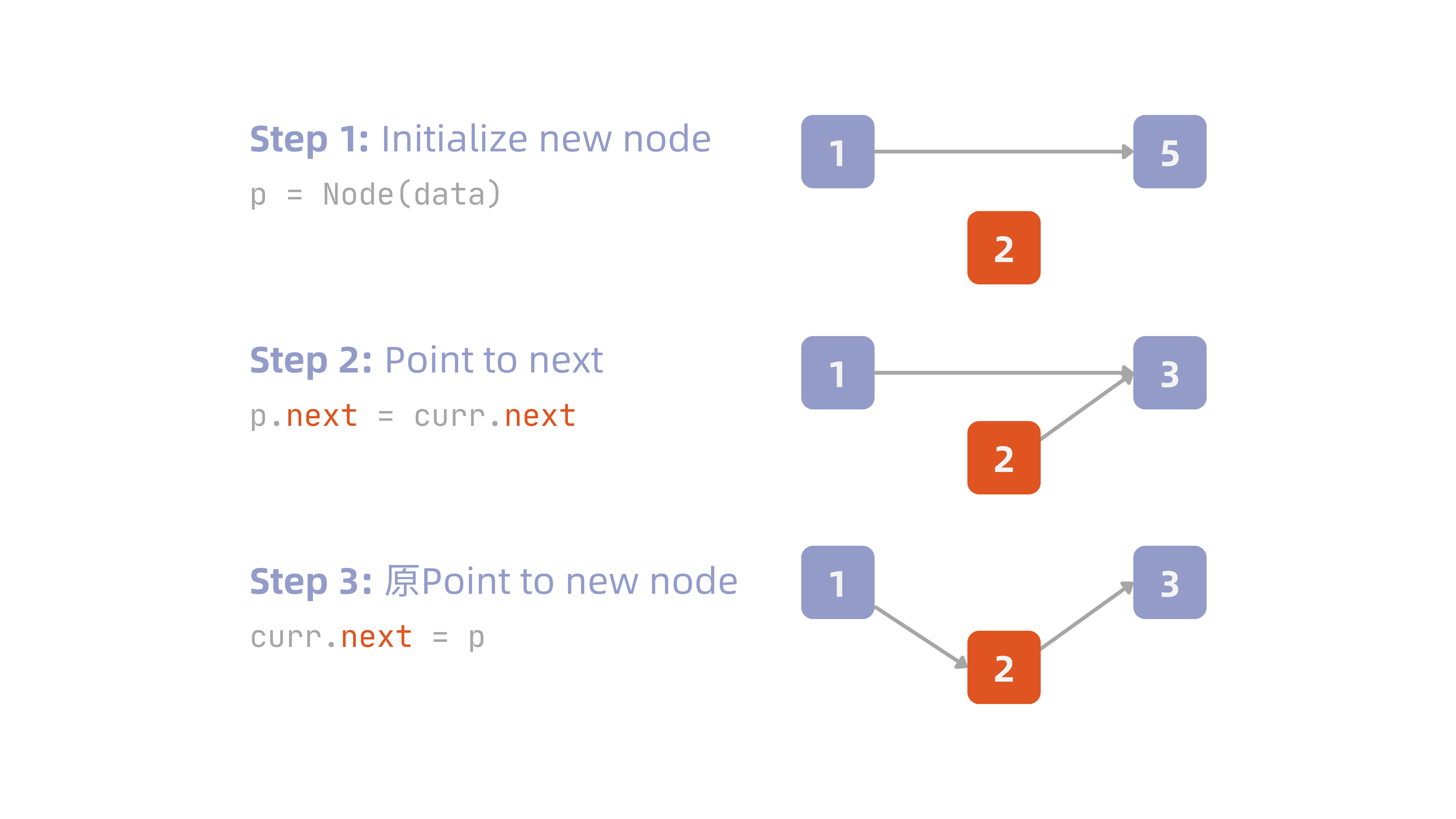
k = 0 needs to be handled separately, because index 0 (the new head) has no previous node to traverse to — that case is handed straight off to insert_at_head. Only for k >= 1 do we traverse to find the predecessor and insert that way.
Say we want node 4 to become index 1 (starting from 1 -> 2 -> 3, 4 is inserted after 1):
1 | head = insert_at(head, 1, 4) |
Inserting at the Tail
This is the opposite case from inserting at the head. Since the tail node has no meaningful next pointer, the only way to move curr to the last node is by traversing — and the way we know this is the last one is that curr.next is None.
1 | def insert_at_tail(head: ListNode | None, data: int) -> ListNode: |
Deleting a ListNode
To delete a node from the list, you first need to find that node’s predecessor, then skip straight over the target node to whatever came after it. Just like insertion, this splits into three cases: deleting the head, deleting a specific node, and deleting the tail.
Deleting the Head
The simplest case. Since the head has no predecessor, all we need to do is make head point to what’s currently the second node:
1 | def delete_at_head(head: ListNode | None) -> ListNode | None: |
Nothing points to the original node 1 anymore, so Python automatically reclaims that memory — no manual deallocation needed.
Deleting a Specific ListNode
To delete the $k$-th node, we first need to traverse to node $k-1$ and stop there (call it curr), then have curr.next skip over the node to be deleted and connect directly to what was x.next.
1 | def delete_at(head: ListNode | None, k: int) -> ListNode | None: |
For example, to delete node 2 — at index 1 — we’d write:
1 | node = delete_at(head, 1) |
Deleting the Tail
Deleting the tail follows the same logic as deleting a middle node — the only difference is that the traversal target becomes the second-to-last node (the one right before the tail), and we set that node’s next to None.
1 | def delete_at_tail(head: ListNode | None) -> ListNode | None: |
Querying a ListNode
Querying a node is considerably simpler than inserting or deleting one. It splits into two cases: querying the $k$-th node and querying by data value.
Querying the $k$-th ListNode
This is almost identical to traversal — the only addition is an index i that tracks how many steps we’ve taken, stopping once we reach step $k$ and returning the current node:
1 | def query_at(head: ListNode | None, k: int) -> ListNode | None: |
Using the earlier list 1 -> 2 -> 3 as an example, querying index 1 (which is node 2):
1 | node = query_at(head, 1) |
If k exceeds the length of the list, curr will reach None, which makes the loop condition false and stops the loop early — so None is returned, meaning no such node exists.
Querying by Data Value
If you don’t know a node’s position and only know the data value you’re looking for, you need to compare each node’s data one by one, until you find a match or reach the end of the list without finding one:
1 | def query_by(head: ListNode | None, data: int) -> ListNode | None: |
Again using 1 -> 2 -> 3 as an example, querying for the node with data 2:
1 | node = query_by(head, 2) |
If that value doesn’t exist in the list, curr will keep going all the way to None, the loop condition becomes false, and None is returned.
Implementing a Singly Linked List
Every operation so far has been a standalone function that takes head as a parameter. Here, we’ll organize them into a single LinkedList class, where head becomes state managed internally by the object, and each operation is rewritten as a method:
1 | class ListNode: |
Compared to the standalone-function version, the content is essentially identical. The only difference is that head — which previously had to be passed in and its return value manually captured on every call — becomes self.head, with the object remembering its own state. The caller no longer needs to worry about capturing a return value, which conveniently fixes the earlier pitfall of forgetting to capture insert_at_head‘s return value, since the method now mutates self.head directly.
Let’s chain a few operations together and see it in action:
1 | ll = LinkedList(ListNode(1)) |
Time Complexity of Each Operation
| Operation | Best Case | Worst Case | Notes |
|---|---|---|---|
| Initialization | $O(1)$ | $O(1)$ | Creating a node and wiring up a pointer are both constant-time steps |
| Traversal | $O(n)$ | $O(n)$ | Every node has to be visited one by one — no shortcuts |
| Insertion | $O(1)$ | $O(n)$ | Inserting at the head needs no traversal; inserting in the middle or at the tail requires traversing to find the position first |
| Deletion | $O(1)$ | $O(n)$ | Deleting the head needs no traversal; deleting in the middle or at the tail requires traversing to find the predecessor first |
| Query | $O(1)$ | $O(n)$ | The smaller the index, or the closer the data sits to the front, the faster; worst case means walking all the way to the end |
Looking back at the singly linked list: even though inserting and deleting a node are constant-time on their own, traversal is $O(n)$, which drags the overall operation down to $O(n)$. The reason is that, unlike an array, a linked list has no formula to compute an address directly.
Doubly Linked List
Unlike a singly linked list, a doubly linked list adds two pointers to each node — one pointing backward, one pointing forward — which makes inserting and deleting around a specific node much more convenient.
First, we can define the node for a doubly linked list:
1 | class DoublyListNode: |
Just like the singly linked list, we organize the operations into a DoublyLinkedList class. The difference is that both the prev and next pointers need to be kept in sync whenever we insert or delete:
1 | class DoublyLinkedList: |
Notice that delete_at here differs from the singly linked version: the singly linked version has to traverse to the predecessor first, because a singly linked node has no way of knowing its own predecessor. The doubly linked version can traverse directly to the target node itself, since prev is available — no need for that extra step.
Circular Linked List
In both the singly and doubly linked lists covered above, the tail node points to None. A circular linked list doesn’t — its tail points back to the head instead, turning the list into a loop (think of it as joining the two ends of an unfolded necklace back together). Using the list from before as an example, converting it into a circular linked list gives 1 -> 2 -> 3 -> 1, implemented like this:
1 | head = ListNode(1) |
From here you can already tell that the original traverse function will fall into an infinite loop. The reason is simple: the tail node no longer points to None, but to the head — so while curr is not None can never break out, and the loop runs forever.
Traversing Nodes
To fix the infinite-loop problem, we need a different stopping condition: since the tail now points back to the head, the loop should end once we hit the head again.
1 | def traverse(head: ListNode | None) -> str: |
The result is still 1 -> 2 -> 3.
Computing the length of a circular linked list also needs special handling:
1 | def length(head: ListNode | None) -> int: |
Inserting a ListNode
Inserting at the head needs separate handling: because a circular list’s tail points back to the head, once the new node becomes the head, the tail also has to be updated to point to it — but there’s no ready-made pointer to the tail, so we have to walk all the way around to find it:
1 | def insert_at_head(head: ListNode | None, data: int) -> ListNode: |
For insertion anywhere else, a circular linked list has no such thing as being out of range — because the structure itself is a closed loop, indices naturally repeat as you go around. So we use length to work out the total length, and normalize $k$ into the range $[0, n)$ with the modulo operator:
1 | def insert_at(head: ListNode | None, k: int, data: int) -> ListNode: |
Using the earlier list as an example: say $k = 100$. Since there are only three nodes, $100 \bmod 3 = 1$, which lands right back on the same node as $k = 1$.
Deleting a ListNode
Deleting the head mirrors inserting at the head: we still need to walk around to find the tail and update it to point to the new head. If only one node is left, deleting it empties the list:
1 | def delete_at_head(head: ListNode | None) -> ListNode | None: |
Deleting anywhere else follows similar logic — again, normalize k first using length:
1 | def delete_at(head: ListNode | None, k: int) -> ListNode | None: |
Querying a ListNode
Querying a node follows the same pattern. Here’s the implementation:
1 | def query_at(head: ListNode | None, k: int) -> ListNode | None: |
If you’re querying by data value instead, you need to cap the loop at exactly one full circuit (controlled via length):
1 | def query_by(head: ListNode | None, data: int) -> ListNode | None: |
Related Topics
Dummy ListNode
Every time we’ve inserted or deleted a node so far, we’ve needed an extra check for the head node — the reason is that the head has no predecessor, which is exactly why we’ve needed if k == 0 and if head is None checks.
The real idea behind a dummy node is this: since the head is missing a predecessor, just conjure one up out of thin air and attach it in front. This node doesn’t hold any real data — it’s purely a placeholder:
1 | dummy = ListNode(0) # the value here doesn't matter |
Now the list is considered to start from dummy, and the actual first piece of data is dummy.next. Insertion and deletion can now be handled with one unified piece of logic — take deletion as an example:
1 | def delete_at(dummy: ListNode, k: int) -> None: |
As mentioned above, since dummy.next is the real data (i.e. the original head), what you return should be dummy.next, not dummy itself.
Reversing a Linked List
Say we’re given the list 1 -> 2 -> 3, and our goal is to reverse it into 3 -> 2 -> 1. How would we go about that?
The core idea is actually simple: to reverse the list, the original head becomes the tail and the tail becomes the head — which implies the original head.next becomes None, and tail.next becomes whatever was the second-to-last node.
Fig 4 simplifies the list down to two nodes for illustration:
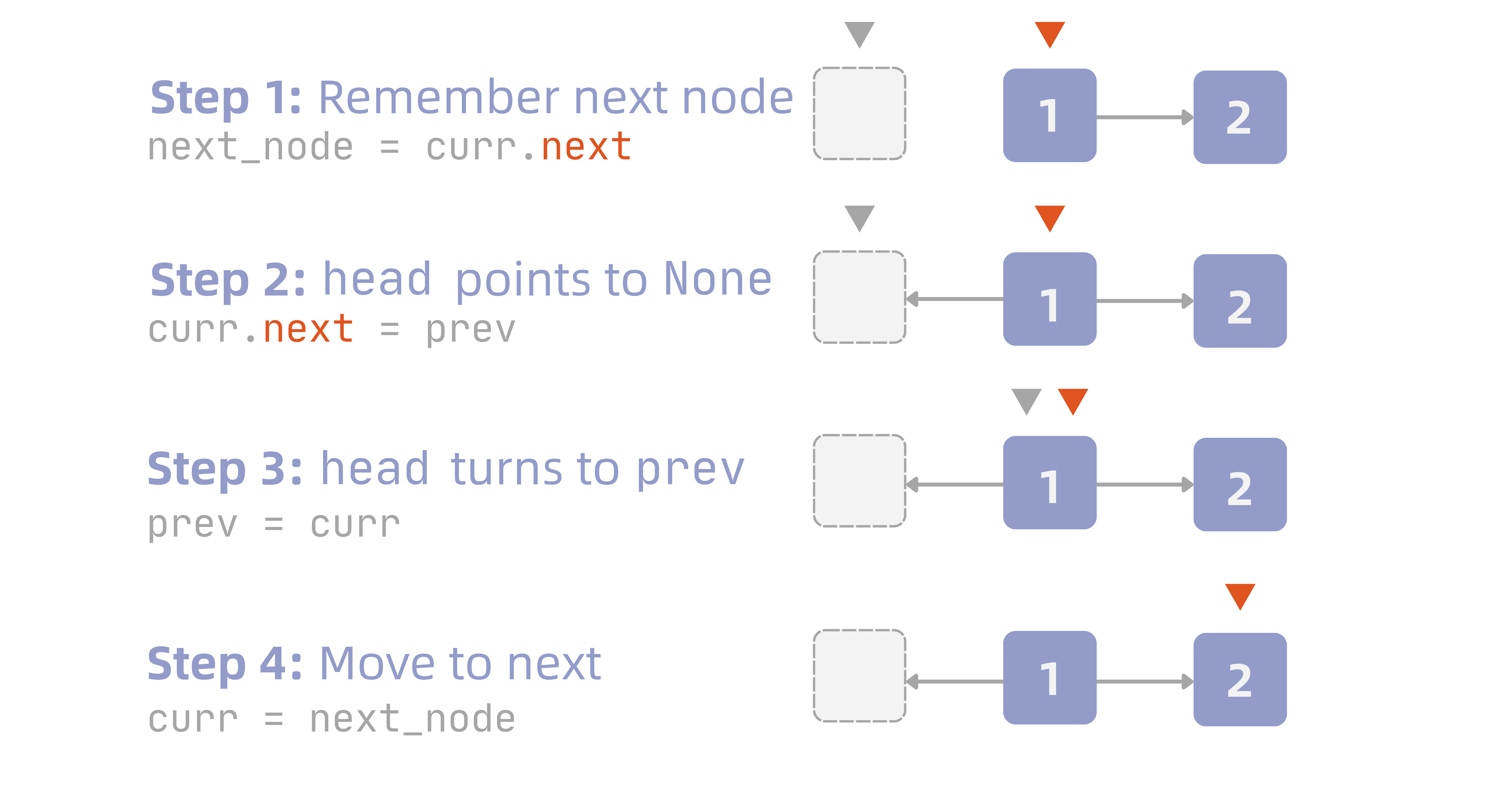
The implementation looks like this:
1 | def reverse(head: ListNode | None) -> ListNode | None: |